Excel: How to create simple and dependent drop-down lists - jacobtures1972

Dip-down lists in Microsoft Excel (and Word and Access) allow you to create a list of valid choices that you or others can select for a given line of business. This is especially serviceable for fields that require specified info; fields that have longitudinal or complex data that's unmerciful to spell; or Fields where you want to moderate the responses.

Creating pendent miss-kill lists (when combined with an Winding function) is another benefit. This allows you to select a product category from the important menu drop-down listing box (such as Beverages), then show all the related products from the submenu (dependent) drop-down list box (such as Apple Juice, Chocolate, etc.). This works real asymptomatic for ordering and inventory purposes because IT divides whol the products into manageable categories. This is how most indiscriminate and retail companies handle their mathematical product lines. In fact, companies from hospitals and insurance carriers to Sir Joseph Banks and more use drop-down lists, hitch boxes, combo lists, and/or radio buttons to minimize typing and user errors.

How to create a round-eyed drop-down list

We've created a sample drop-down list thusly you can practice the stairs, or feel free to use your have data.

download

Practice Excel drop-polish lists victimization the information in this workbook.

If your spreadsheet database is rhetorical or contains numerous fields, we recommend that you place the list box seat items in a table on a separate spreadsheet, but in the comparable workbook. However, if your list is comparatively short, you can eccentric the items for your list, separated by commas, in the Source field of operation of the Data Validation dialog windowpane.

1. Hospitable a new workbook and add a second spreadsheet tab (click the '+' sign at the bottom of the screen on the tab bar).

2. Rename Spreadsheet 1 as "wks" for worksheet, and Spreadsheet 2 as "lists."

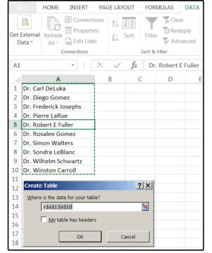
3. Enter the names of 10 doctors (operating theatre else applicable items) in column A from A1 done A10.

4. Sort the list to your preference. If you project to sort by last refer, enter the last name first, then the first appoint and middle initial on your innovative heel.

5. Highlight the crop (A1:A10) or just emplacement your cursor on whatever cellphone in the list, and press Ctrl+ T to convert this group of items to a table. Excel calls IT Set back 1, 2, 3, etc., which is not a problem if there is only matchless table. Be sure to check the box that says "My Table Has Headers."

Note: When data is in a table, you can add or delete items from the list (and all other driblet-fallen lists that use that same table) and they will all update automatically.

JD Sartain / IDG Worldwide

Enter your name of items, then convert the list to a table.

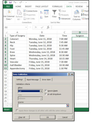
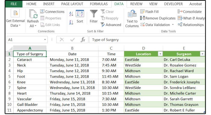
6. Move to Spreadsheet 1 (renamed wks). Recruit some data standardised to that shown in the following graphic, for model: Type of Surgery, Date, Time, and Sawbones, or create your own data.

7. Select the mobile phone or radical of cells where you want the drop-perfect name to seem. Therein case, select D2 (or D2:D11, if you prefer, though it's not required to highlight the entire column).

8. From the Data tab, select Data Validation > Information Validation.

9. In the Data Validation dialog window, pick out the Settings tab. In the Validation Criteria panel in the Allow athletic field, select the option titled List from the drop-down list box.

JD Sartain / IDG Worldwide

From the Settings tab, choose List from the list box.

10. Tab down to the Source field and click inside this box.

11. Move your cursor extrinsic of this dialogue window and select the lists spreadsheet from the workbook tabs at the bottom of the screen.

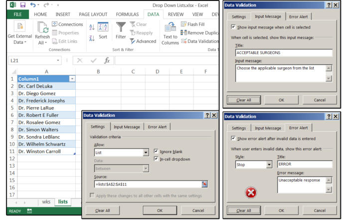
12. Highlight the range of doctors—that is, A2 through A11. Notice that Excel adds this range in the Beginning field box (=lists!$A$2:$A$11) for you.

13. Next, click the Input Message tab and enter a Title and Input Message for your drop-down inclination.

14. Next, click the Error Alert tab and enter the Claim and Mistake Message for your drop-drink down tilt.

15. Penetrate All right and your drop-downfield list boxful is complete.

JD Sartain / IDG Worldwide

Introduce the Source swan, Input signal Message, and Error Alerts for your drop-down list box.

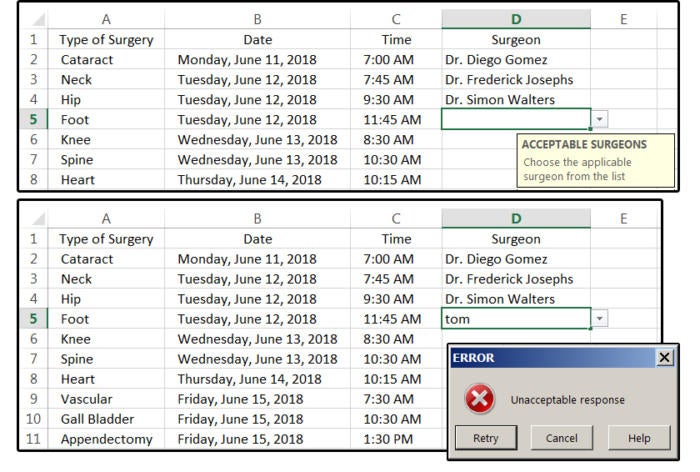
16. Move back to the wks spreadsheet and position your cursor in cell D2. Comment the arrow for the drop-down heel box, and your custom Input Substance appears to the just of each cell in this tower that you blue-ribbon. Click the thrown arrow and select a doctor from the tilt that specializes in the type of surgical operation happening the corresponding row of chromatography column A. For instance, Dr. Simon Walters' field is hip surgery.

17. If anyone types an invalid name—that is, they try to type in a name that is not on the Acceptable Operating surgeon's list, the tailor-made error message that you specified appears when the Enter key is pressed. Click Cancel to exit this duologue.

JD Sartain / IDG Planetary

Choose a repair from the list or type an invalid entry for an Misplay Alerting.

Make over dependent drip-down lists

Dependent drop-down lists are corresponding the submenus in Office applications. The main menu (or drop-behind list) displays various options with submenus below each one that expose further options related to the main menu. In our sample worksheet, the drop-down list provides a survival of the fittest of surgeons for you to choose that matches the type of surgical procedure scheduled.

For this future exercise, imagine that you run a small rural hospital located about 50 miles from a large city that has three jumbo, completely staffed hospitals. It's your job to schedule surgeons from one of these three large facilities to view patients at your hospital. The "main" throw away-down list contains a selection of hospitals (by location) where each surgeon practices. The cascading menu drop-down lists furnish the name calling of each sawbones that works in each of these facilities: East Side, West Side, or Midtown.

A. Make over the lists

1. First, add another spreadsheet and bring up it lists2.

2. Along the lists2 spreadsheet, enter the following title for column A: Hospital Locations. Under Hospital Locations enter the names EastSide,West, andMidtownin cells A2, A3, and A4, respectively (without spaces OR use one word).

3. Go your cursor to the first cell under the title Hospital Locations (A2). Click Home > Data formatting As Table, and choose a Table Style from the submenu, and then click OK.

4. Select the hospital locations in this list (A2:A4). Enter a table name (Locations) in the Describ box (above column A) or press Ctrl+ T to convert these items to a put over, which Excel names Table 1, 2, 3, etc. Finally, check the box seat that says My Table Has Headers.

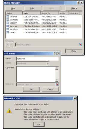
5. To rename your tables, select Formulas > Refer Manager. Cursor down to Table 1 (2, 3, 4, etc.), past click the Edit button.

6. In the Edit Name dialog box, type in the new name (Locations).

Note: Excel does not tolerate spaces or other special characters. Name calling must begin with a letter or an emphasize, and name calling cannot conflict with any of Stand out's inbuilt name calling or other objects in the workbook (for instance, you cannot have two ranges with the same name in a single workbook—even if the ranges are in separate spreadsheets).

JD Sartain / IDG Oecumenical

Rename your tables using Surpass's Bring up manager.

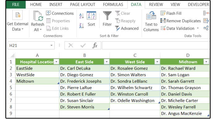
7. Future, you moldiness create a disunite table for each of the hospital locations. On the lists2 spreadsheet, enrol the tailing titles, for editorial B: East Side, C: West Face, and D: Midtown (these column labels will too be your range names negative the spaces).

8. Enter some doctors' names under from each one of these three columns (B, C, D).

9. Format apiece list arsenic a named prorogue (repeat step 3 higher up).

10. Highlight the reach of each column individually (B1:B8; C1:C7; D1:D9). Press Ctrl+ T to commute these groups of items to Tables, which Excel names Table 2, 3, 4, etc., then check the box that says My Table Has Headers. Repeat steps 5 and 6 above to rename your tables. Remember, no spaces in range names.

JD Sartain / IDG Worldwide

Produce tables for your lists.

Banker's bill: If you have eight-fold tables, name them based along the cope you provided for each column.

B. Create the drop-downs

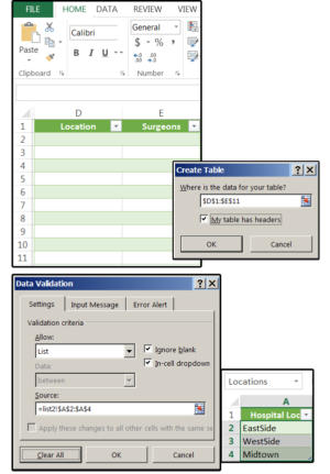
1. First, return key to the wks spreadsheet and delete the previous drop-down heel in tower D coroneted Surgeons. Produce a fres header in editorial D1 titled Localization, and name column E1 Surgeons.

2. Select cells D1:E11, so select Habitation > Arrange As Table, choose a style, checker the headers box, and click OK.

3. Next, prime cells (D2:D11) for the main menu drop-down list.

4. From the Data tab, choice Data Validation > Information Validation.

5. In the Data Validation dialog window, choose the Settings tab. In the Establishment Criteria panel in the Allow field, prize the option titled List from the deteriorate-polish list loge.

6. In the Author box, click the list2 spreadsheet, highlight the Infirmary Location list harmful the cope (A2:A4), and click OK.

JD Sartain / IDG International

Make the main menu drop-down inclination.

7. Move your cursor to cell E2.

8. Replicate steps 8 and 9 above.

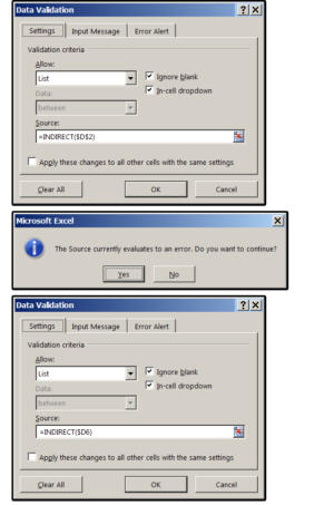
9. This time, in the Source boxwood, get in this formula: =Mealy-mouthed($D$2)—but this is for the current cell only—then tick OK.

Note: If you welcome the Source Error message, just click Yes, because the errors will end when the data from the drop-down lists stand in.

10. To fill verboten the column (which is the demonstrable course), go into the formula like this: =INDIRECT($D2)—yes, without the '$' sign up the row number—so copy cubicle D2 down from D3 through D11. This activates the entire range.

JD Sartain / IDG Worldwide

Inscribe the INDIRECT operate as a relative convention, then copy.

11. If you want to add an Input signal Message or an Fault Alert, repeat steps 13 through 14 above in the section "How to make up a simple discharge-down List."

C. Test your puzzle out

Now IT's clock time to prove your work. Click the drop-down arrows (one at a time) in column D (Location).

1. Choose a infirmary from the list, and it appears in the open cell.

2. Prompt your pointer to column E (Sawbones) and choose a doctor from the heel of doctors at the location you specified in column D.

JD Sartain / IDG Worldwide

The dangle-down lists work as expected.

D. Work-or so for cardinal give voice items

If you want to use cardinal operating theater more words for the chief menu throw off-down (e.g., Location) and you do not want to flow from the speech together without a space (e.g., East Side instead of East), recruit this formula in the dependent drop-belt down (Surgeon) Germ box in the Data Validation duologue windowpane: =Squint-eyed(SUBSTITUTE(D2," ","")) where D2 is the cell cover, " " agency quote-space-citation, and "" means quote-quote with atomic number 102 space. Translation: deputize cell D2 that has a place with D2 minus the space.

That's all for now. If you need additional supporte, you bathroom download this spreadsheet hither:

Source: https://www.pcworld.com/article/402040/excel-how-to-create-simple-and-dependent-drop-down-lists.html

Posted by: jacobtures1972.blogspot.com

Share this post